
Case Three: Implementing Your Own Model with benco init
We believe that the fastest way to learn is "Learn by Doing" (learning by doing), so we use several cases to help users get started quickly.
Overall, IMDL-BenCo helps you quickly complete the development of image tampering detection scientific research projects through command line calls similar to git and conda. If you have learned front-end technologies such as vue, understanding the design pattern of IMDLBenCo according to vue-cli will be very easy.
Regardless, please refer to Installation to complete the installation of IMDL-BenCo first.
Motivation of This Chapter
To ensure that you can flexibly create your own models, this chapter will help you understand the design patterns and interface paradigms of IMDL-BenCo. We will introduce each part step by step according to the usage process.
Introducing All Design Patterns
Generating Default Scripts
Under a clean working path, executing the following command line instruction will generate all the scripts needed for creating your own model and testing. As a default instruction, omitting the base will also execute the same command.
benco init base
benco init
After normal execution, you will see the following files generated under the current path, and their uses are as commented:
.
├── balanced_dataset.json       # Stores the dataset path organized according to Protocol-CAT
├── mymodel.py                  # The core model implementation
├── README-IMDLBenCo.md         # A simple readme
├── test_datasets.json          # Stores the test dataset path
├── test_mymodel.sh             # The shell script for running tests with parameters
├── test.py                     # The actual Python code for the test script
├── test_robust_mymodel.sh      # The shell script for running robustness tests with parameters
├── test_robust.py              # The actual Python code for robustness tests
├── train_mymodel.sh            # The shell script for running training with parameters
└── train.py                    # The actual Python code for the training script
Special Attention
If the scripts have been generated and some modifications have been made, please be very careful when calling benco init for the second time. IMDLBenCo will cover the files one by one after asking, and if you operate incorrectly, it may cause you to lose your existing modifications. Be careful. It is recommended to use git version control to avoid losing existing code due to this operation.
Model File Design Pattern
IMDLBenCo needs to organize the model files in a certain format to ensure that the entry can align with the DataLoader and the exit can align with the subsequent Evaluator and Visualize tools.
After executing benco init, a model with the simplest single-layer convolution is generated in mymodel.py by default. You can quickly view its content through the Github link to mymodel.py.
from IMDLBenCo.registry import MODELS
import torch.nn as nn
import torch

@MODELS.register_module()
class MyModel(nn.Module):
    def __init__(self, MyModel_Customized_param:int, pre_trained_weights:str) -> None:
        """
        The parameters of the `__init__` function will be automatically converted into the parameters expected by the argparser in the training and testing scripts by the framework according to their annotated types and variable names.

        In other words, you can directly pass in parameters with the same names and types from the `run.sh` script to initialize the model.
        """
        super().__init__()

        # Useless, just an example
        self.MyModel_Customized_param = MyModel_Customized_param
        self.pre_trained_weights = pre_trained_weights

        # A single layer conv2d
        self.demo_layer = nn.Conv2d(
            in_channels=3,
            out_channels=1,
            kernel_size=3,
            stride=1,
            padding=1,
        )

        # A simple loss
        self.loss_func_a = nn.BCEWithLogitsLoss()

    def forward(self, image, mask, label, *args, **kwargs):
        # simple forwarding
        pred_mask = self.demo_layer(image)

        # simple loss
        loss_a = self.loss_func_a(pred_mask, mask)
        loss_b = torch.abs(torch.mean(pred_mask - mask))
        combined_loss = loss_a + loss_b


        pred_label = torch.mean(pred_mask)

        inverse_mask = 1 - mask

        # ----------Output interface--------------------------------------
        output_dict = {
            # loss for backward
            "backward_loss": combined_loss,
            # predicted mask, will calculate for metrics automatically
            "pred_mask": pred_mask,
            # predicted binaray label, will calculate for metrics automatically
            "pred_label": pred_label,

            # ----values below is for visualization----
            # automatically visualize with the key-value pairs
            "visual_loss": {
                # keys here can be customized by yourself.
                "predict_loss": combined_loss,
                'loss_a' : loss_a,
                "I am loss_b :)": loss_b,
            },

            "visual_image": {
                # keys here can be customized by yourself.
                # Various intermediate masks, heatmaps, and feature maps can be appropriately converted into RGB or single-channel images for visualization here.
                "pred_mask": pred_mask,
                "reverse_mask" : inverse_mask,
            }
            # -------------------------------------------------------------
        }

        return output_dict


if __name__ == "__main__":
    print(MODELS)
Introducing the design requirements of IMDLBenCo's model file from top to bottom:
- Line 5:
@MODELS.register_module()- Registers the model to IMDLBenCo's global registry based on the registration mechanism, making it easy for other scripts to quickly call the class through strings.
- If you are not familiar with the registration mechanism, a one-sentence explanation is: It automatically maintains a dictionary mapping from strings to corresponding class mappings, making it easy to "freely" pass parameters.
- In actual use, by passing the registered "class name identical string" to the
--modelfunction of the shell script that starts training, the framework can load the corresponding custom or built-in model. For details, please refer to this link.
- Lines 29 and 37: Loss functions must be defined in the
__init__()orforward()functions - Line 31: Defining the forward function
def forward(self, image, mask, label, *args, **kwargs):- It is necessary to include
*args, **kwargsrequired for Python function unpacking to receive unused parameters.- If you are not familiar with it, please refer to Python Official Documentation-4.8.2. Keyword Arguments, Python Official Documentation Chinese Version-4.8.2 Keyword Arguments
- The parameter variable names must be exactly the same as the field names contained in the dictionary
data_dictreturned byabstract_dataset.py. The default fields are shown in the table below:Key Name Meaning Type image Input original image Tensor(B,3,H,W) mask Mask of the prediction target Tensor(B,1,H,W) edge_mask After erosion (erosion) and dilation (dilation) based on the mask, only the boundary is white, which is used for various models that need boundary loss functions. To reduce computational overhead, the corresponding dataloader will only return this key-value pair for the model's forward()function when the--edge_mask_width 7parameter is passed in the trainingshell, refer to the shell and model forward function ofIML-ViT.
If you do not need the boundary mask to calculate subsequent losses, you do not need to pass it in the shell, nor do you need to prepare a parameter namededge_maskin the model'sforward()function, refer to the shell and model forward function ofObjectFormer.Tensor(B,1,H,W) label Image-level prediction of zero-one labels Tensor(B,1) shape The shape of the image after padding or resizing Tensor(B,2), two dimensions each with one value, representing H and W respectively original_shape The shape of the image when it was first read Tensor(B,2), two dimensions each with one value, representing H and W respectively name The path and filename of the image str shape_mask In the case of padding, only the pixels inside this mask that are 1 are calculated as the final metric, 1 defaults to a square area the same size as the original image Tensor(B,1,H,W) - For different tasks, you can take these fields as needed and input them into the model for use.
- In addition, for the Jpeg-related image materials needed by CAT-Net, we have designed the post-processing function
post_functo generate more content based on the existing fields. At this time, it is also necessary to ensure that the corresponding forward function's fields are aligned. Custom models with similar needs can also use this pattern to introduce other modal information in the dataloader. The following is a case of CAT-Net:- Github link to
cat_net_post_function, you can see that it includes two additional fieldsDCT_coefandq_tablesfor the model to input additional modalities - Github link to
cat_net_model, theforwardfunction's parameter list needs to have corresponding fields to receive the above additional input information.
- Github link to
- It is necessary to include
- Lines 36 to 38: All loss functions must be calculated in the
forwardfunction - Lines 45 to 70: The dictionary of output results. Very important!, the function of each field in the dictionary is introduced as follows:
Key Meaning Type backward_loss The loss function directly used for backpropagation Tensor(1) pred_mask The predicted mask, which will be directly used for subsequent metric calculations Tensor(B,1,H,W) pred_label The predicted zero-one label, which will be directly used for subsequent metric calculations Tensor(B,1) visual_loss Pass in the scalars that need to be visualized. You can name any number, any name of keys and pass in the corresponding scalars, which will be automatically visualized according to the Key name later Dict() visual_image Pass in the images, feature maps, various masks that need to be visualized. You can name any number, any name of keys and pass in the corresponding Tensors, which will be automatically visualized according to the Key name later Dict() - Be sure to organize according to this format to integrate normally into subsequent metric calculations, visualization, etc.
Step-by-Step Comprehensive Tutorial
We will use the ConvNeXt as a model, CASIAv2 as the training set, and CASIAv1 as the test set to guide you through the process of designing, training, and testing your own new model with IMDL-BenCo from start to finish.
Downloading Datasets
This repository provides an index directory, introduction, and errata for the current mainstream tampering detection datasets. Please refer to the Tampering Detection Dataset Index section.
Note
Many tampering detection datasets are manually annotated and collected, which leads to many errors, so necessary corrections are essential. Common errors include:
- Inconsistent image and mask resolutions;
- Extra images without corresponding masks;
- Obvious misalignment between images and masks;
More information on corrections can be found in this IML-Dataset-Corrections repository.
- CASIAv2 download link:
- Please refer to the
Fixed groundtruth downloadingsection in Sunnyhaze's repository to download the complete dataset.
- Please refer to the
- CASIAv1 download link:
- Download the original dataset images from the cloud storage link in the Readme of namtpham's repository.
- Please clone this repository to download the corresponding masks for the images.
git clone https://github.com/namtpham/casia1groundtruth
Organizing Datasets into a Format Readable by IMDL-BenCo
Please refer to the Dataset Preparation Section for specific format requirements.
- The downloaded CASIAv2 dataset is already organized in the
ManiDatasetformat and can be used directly after extraction. - The downloaded CASIAv1 dataset requires further processing. We provide two methods here,
JsonDatasetandManiDataset.
First, after extracting the original dataset CASIA 1.0 dataset provided by this repository, you can see the following files:
.
├── Au.zip
├── Authentic_list.txt
├── Modified Tp.zip
├── Modified_CopyMove_list.txt
├── Modified_Splicing_list.txt
├── Original Tp.zip
├── Original_CopyMove_list.txt
└── Original_Splicing_list.txt
Due to some filename errors from the official CASIA, this repository has corrected these naming errors. In fact, we only need to extract the modified Modified Tp.zip, which results in:
└── Tp
    ├── CM
    └── Sp
Where CM contains the tampered images corresponding to Copy-move; and SP contains the tampered images corresponding to Splicing. There should be a total of 921 images in theory.
Important!
According to the errata repository, there is an extra image without a corresponding mask, namely: CASIA1.0/Modified Tp/Tp/Sp/Sp_D_NRN_A_cha0011_sec0011_0542.jpg. We recommend removing this image from the dataset before proceeding with further processing.
Additionally, after extracting the CASIA 1.0 groundtruth, you get:
.
└── CASIA 1.0 groundtruth
    ├── CM
    ├── CopyMove_groundtruth_list.txt
    ├── FileNameCorrection.xlsx
    ├── Sp
    └── Splicing_groundtruth_list.txt
Similarly, CM contains the masks corresponding to Copy-move; and SP contains the masks corresponding to Splicing. There should be 920 images in theory. To ensure one-to-one correspondence between images and masks, please remove the extra image from the tampered images as mentioned above.
Next, we demonstrate how to organize CASIAv1 into a dataset readable by IMDL-BenCo in two ways.
Organizing Dataset with JsonDataset
You can generate a JSON file readable by IMDL-BenCo by executing the following Python script in the set path:
import os
import json

def collect_image_paths(root_dir):
    """Collect the relative and absolute paths of all image files in the directory"""
    image_exts = {'.jpg', '.jpeg', '.png', '.bmp', '.tif', '.tiff', '.webp'}
    image_paths = []
    pwd = os.getcwd()
    for dirpath, _, filenames in os.walk(root_dir):
        for filename in filenames:
            file_ext = os.path.splitext(filename)[1].lower()
            if file_ext in image_exts:
                abs_path = os.path.normpath(os.path.join(dirpath, filename))
                image_paths.append(os.path.join(pwd, abs_path))
    return image_paths

def generate_pairs(image_root, mask_root, output_json):
    # Collect image paths
    image_dict = collect_image_paths(image_root)
    print("Number of images found:", len(image_dict))
    mask_dict = collect_image_paths(mask_root)
    print("Number of masks found:", len(mask_dict))
    assert len(image_dict) == len(mask_dict), "The number of images {} and the number of masks {} do not match!".format(len(image_dict), len(mask_dict))
    # Generate pairing list
    pairs = [
        list(pairs)
        for pairs in zip(sorted(image_dict), sorted(mask_dict))
    ]
    print(pairs)

    # Save as JSON file
    with open(output_json, 'w') as f:
        json.dump(pairs, f, indent=2)

    print(f"Successfully generated {len(pairs)} pairs of paths, results saved to {output_json}")
    return pairs

if __name__ == "__main__":
    # Configure paths (modify according to actual situation)
    IMAGE_ROOT = "Tp"
    MASK_ROOT = "CASIA 1.0 groundtruth"
    OUTPUT_JSON = "CASIAv1.json"

    # Execute generation
    result_pairs = generate_pairs(IMAGE_ROOT, MASK_ROOT, OUTPUT_JSON)

    # Print the last 5 pairs as an example to verify alignment
    print("\nLast five example pairs:")
    for pair in result_pairs[-5:]:
        print(f"Image: {pair[0]}")
        print(f"Mask:  {pair[1]}\n")
For example, I generated a json file like this:
[
  [
    "/mnt/data0/xiaochen/workspace/IMDLBenCo_pure/guide/Tp/CM/Sp_S_CND_A_pla0016_pla0016_0196.jpg",
    "/mnt/data0/xiaochen/workspace/IMDLBenCo_pure/guide/CASIA 1.0 groundtruth/CM/Sp_S_CND_A_pla0016_pla0016_0196_gt.png"
  ],
   ......
]
Subsequently, you can write the absolute path of this json file as the test set parameter in the shell, for example:
/mnt/data0/xiaochen/workspace/IMDLBenCo_pure/guide/CASIAv1.json
Note that, if you build your own dataset with real images later, you need to write the path of the mask for real images as the string Negative when building the JSON script. This way, Benco will treat this image as a real image with a pure black mask. For example, if you want to use the above image as a real image, the json should be organized like this:
[
  [
    "/mnt/data0/xiaochen/workspace/IMDLBenCo_pure/guide/Tp/CM/Sp_S_CND_A_pla0016_pla0016_0196.jpg",
    "Negative"
  ],
   ......
]
Organizing Dataset with ManiDataset
Very simple, find a clean path to store the dataset and create a folder named CASIAv1, then create two subfolders with the following names:
└── CASIAv1
    ├── Tp
    └── Gt
Then copy the 920 tampered images to the Tp path and copy the 920 masks to the Gt path. Subsequently, you can write the path of this folder as the test set parameter in the shell, for example:
/mnt/data0/xiaochen/workspace/IMDLBenCo_pure/guide/CASIAv1
Adjusting the Design of Your Own Model under benco init
First, we need to execute benco init to generate all the required files and scripts. A brief introduction to the generated files has been given in the first half of this chapter.
To customize your own model, you need to modify mymodel.py. We will first provide the modified code and then introduce the important parts.
from IMDLBenCo.registry import MODELS
import torch.nn as nn
import torch
import torch.nn.functional as F
import timm

class ConvNeXtDecoder(nn.Module):
    """Adapted ConvNeXt feature decoder"""
    def __init__(self, encoder_channels=[96, 192, 384, 768], decoder_channels=[256, 128, 64, 32]):
        super().__init__()
        # Use transposed convolution for upsampling step by step
        self.decoder = nn.Sequential(
            nn.ConvTranspose2d(encoder_channels[-1], decoder_channels[0], kernel_size=4, stride=4),  # 16x16 -> 64x64
            nn.GELU(),

            nn.ConvTranspose2d(decoder_channels[0], decoder_channels[1], kernel_size=4, stride=4),  # 64x64 -> 256x256
            nn.GELU(),

            nn.Conv2d(decoder_channels[1], decoder_channels[2], kernel_size=3, padding=1),
            nn.GELU(),

            nn.Conv2d(decoder_channels[2], decoder_channels[3], kernel_size=3, padding=1),
            nn.GELU(),

            nn.Conv2d(decoder_channels[3], 1, kernel_size=1)
        )

    def forward(self, x):
        return self.decoder(x)

@MODELS.register_module()
class MyConvNeXt(nn.Module):
    def __init__(self) -> None:
        super().__init__()

        # Initialize ConvNeXt-Tiny backbone network
        self.backbone = timm.create_model(
            "convnext_tiny",
            pretrained=True,
            features_only=True,
            out_indices=[3],  # Take the last feature map (1/32 downsampling)
        )

        # Segmentation decoder
        self.seg_decoder = ConvNeXtDecoder()

        # Classification head
        self.cls_head = nn.Sequential(
            nn.AdaptiveAvgPool2d(1),
            nn.Flatten(),
            nn.Linear(768, 1)  # ConvNeXt-Tiny's last channel count is 768
        )

        # Loss functions
        self.seg_loss = nn.BCEWithLogitsLoss()
        self.cls_loss = nn.BCEWithLogitsLoss()

    def forward(self, image, mask, label, *args, **kwargs):
        # Feature extraction
        features = self.backbone(image)[0]  # Get the last feature map [B, 768, H/32, W/32]

        # Segmentation prediction
        seg_pred = self.seg_decoder(features)
        seg_pred = F.interpolate(seg_pred, size=mask.shape[2:], mode='bilinear', align_corners=False)

        # Classification prediction
        cls_pred = self.cls_head(features).squeeze(-1)

        # Calculate losses
        seg_loss = self.seg_loss(seg_pred, mask)
        cls_loss = self.cls_loss(cls_pred, label.float())
        combined_loss = seg_loss + cls_loss

        # Build output dictionary
        output_dict = {
            "backward_loss": combined_loss,
            "pred_mask": torch.sigmoid(seg_pred),
            "pred_label": torch.sigmoid(cls_pred),

            "visual_loss": {
                "total_loss": combined_loss,
                "seg_loss": seg_loss,
                "cls_loss": cls_loss
            },

            "visual_image": {
                "pred_mask": seg_pred,
            }
        }
        return output_dict

if __name__ == "__main__":
    # Test code
    model = MyConvNeXt()
    x = torch.randn(2, 3, 512, 512)
    mask = torch.randn(2, 1, 512, 512)
    label = torch.randint(0, 2, (2,)).float()  # Note that the label dimension is adjusted to [batch_size]
    output = model(x, mask, label)
    print(output["pred_mask"].shape)  # torch.Size([2, 1, 512, 512])
    print(output["pred_label"].shape) # torch.Size([2])
We first renamed the model class to class MyConvNeXt(nn.Module). Only the entry of the complete model needs to add the @MODELS.register_module() decorator to complete global registration. The previous submodule class ConvNeXtDecoder(nn.Module): does not need to be called directly by IMDL-BenCo, so there is no need to register it or maintain a special interface.
It can be noted that the loss functions are defined inside the __init__() function and calculated in the forward() function.
The final output dictionary returns the following according to the interface format:
backward_loss, the loss function;pred_mask, the pixel-level prediction result of the segmentation head, which is a 0~1 probability map and will be automatically used to calculate all pixel-level metrics, such aspixel-level F1;pred_label, the image-level prediction result of the classification head, which is a 0~1 probability value and will be automatically used for all image-level metrics, such asimage-level AUC;visual_loss, a dictionary of scalar loss functions for visualization, plotting a line chart for each scalar according to the numerical changes per Epoch;visual_image, a dictionary of prediction tensors for observing the predicted mask, displaying all tensors in the dictionary through the tensorboard API.
Important
This dictionary is an important interface for IMDL-BenCo to automatically complete calculations and visualizations. Please be sure to master it.
Modify Other Scripts
First, since some information in mymodel.py has been modified, you need to modify the corresponding file interfaces. Mainly includes the following places:
- The beginning of
train.py,test.py, andtest_robust.pyregarding the model'simportis modified to the corresponding model name- Originally
from mymodel import MyModel, here it is modified to the new model namefrom mymodel import MyConvNeXt - Of course, if you change the file name of
mymodel.py, it is also possible, as long as the corresponding import is consistent. - If not imported, IMDL-BenCo will not be able to find the corresponding model during subsequent training.
- Originally
Important TODOs Awaiting Your Modifications
There are many TODO comments in the files train.py, test.py, and test_robust.py, which are intended to encourage you to make active modifications.
For example, if you want to introduce metrics such as Pixel-AUC, you will also need to manually modify the corresponding TODO sections to achieve this.
- The script
train_mymodel.shis the shell script to start training and definitely needs to be modified.- Change the
--modelfield toMyConvNeXt, the model will automatically match the corresponding model based on this string from the registered classes. - Since this model's
__init__()function has no parameters, the two redundant parameters--MyModel_Customized_paramand--pre_trained_weightsshown in this example can be directly deleted. The documentation for this technique is in the Passing nn.Module Hyperparameters through Shell section. - Modify the
--data_pathfield to the prepared training set path. - Modify the
--test_data_pathfield to the previously prepared test set path. - Modify other training hyperparameters to match your device requirements, computational efficiency, etc. Here is an example of a modified
train_mymodel.sh.
- Change the
base_dir="./output_dir"
mkdir -p ${base_dir}

CUDA_VISIBLE_DEVICES=0,1 \
torchrun  \
    --standalone    \
    --nnodes=1     \
    --nproc_per_node=2 \
./train.py \
    --model MyConvNeXt \
    --world_size 1 \
    --batch_size 32 \
    --test_batch_size 32 \
    --num_workers 8 \
    --data_path /mnt/data0/public_datasets/IML/CASIA2.0 \
    --epochs 200 \
    --lr 1e-4 \
    --image_size 512 \
    --if_resizing \
    --min_lr 5e-7 \
    --weight_decay 0.05 \
    --edge_mask_width 7 \
    --test_data_path "/mnt/data0/public_datasets/IML/CASIA1.0" \
    --warmup_epochs 2 \
    --output_dir ${base_dir}/ \
    --log_dir ${base_dir}/ \
    --accum_iter 8 \
    --seed 42 \
    --test_period 4 \
2> ${base_dir}/error.log 1>${base_dir}/logs.log
Here I have two graphics cards, so I set CUDA_VISIBLE_DEVICES=0,1 and --nproc_per_node=2, you can modify it to the number supported by your device and the corresponding graphics card number.
Conduct Training
Then, execute the following command in the working directory to start training:
sh train_mymodel.sh
If there is no output, don't panic, in order to save logs, all outputs and errors are redirected to files.
If run correctly, a folder named output_dir_xxx or eval_dir_xxx will be generated in the current path, which outputs three logs, one is the normal standard output logs.log, one is warnings and errors error.log. There is also an independent log file specifically for statistical vectors log.txt
If the model runs normally, you should be able to see the model continuously iterating and outputting new logs at the end of logs.log:
[01:51:01.408908] Epoch: [99] Total time: 0:00:47 (0.5883 s / it)
[01:51:08.313768] Averaged stats: lr: 0.000051  total_loss: 0.0379 (0.0425)  seg_loss: 0.0379 (0.0425)  cls_loss: 0.0000 (0.0000)
[01:51:08.319097] log_dir: ./output_dir/
[01:51:12.473905] Epoch: [100]  [ 0/80]  eta: 0:05:32  lr: 0.000051  total_loss: 0.0415 (0.0415)  seg_loss: 0.0415 (0.0415)  cls_loss: 0.0000 (0.0000)  time: 4.1538  data: 2.5060  max mem: 12775
[01:51:23.468235] Epoch: [100]  [20/80]  eta: 0:00:43  lr: 0.000051  total_loss: 0.0383 (0.0426)  seg_loss: 0.0383 (0.0426)  cls_loss: 0.0000 (0.0000)  time: 0.5496  data: 0.0083  max mem: 12775
[01:51:34.303514] Epoch: [100]  [40/80]  eta: 0:00:25  lr: 0.000051  total_loss: 0.0354 (0.0406)  seg_loss: 0.0354 (0.0406)  cls_loss: 0.0000 (0.0000)  time: 0.5417  data: 0.0002  max mem: 12775
[01:51:45.128389] Epoch: [100]  [60/80]  eta: 0:00:12  lr: 0.000050  total_loss: 0.0304 (0.0401)  seg_loss: 0.0304 (0.0401)  cls_loss: 0.0000 (0.0000)  time: 0.5412  data: 0.0002  max mem: 12775
[01:51:55.408163] Epoch: [100]  [79/80]  eta: 0:00:00  lr: 0.000050  total_loss: 0.0366 (0.0394)  seg_loss: 0.0366 (0.0394)  cls_loss: 0.0000 (0.0000)  time: 0.5409  data: 0.0001  max mem: 12775
According to the above settings, this example occupies two graphics cards, with each card occupying 4104M of memory.
Here is a recommended tool to check graphics card usage, gpustat. After installing pip install gpustat and executing gpustat in the command line, you can easily view the graphics card usage and corresponding users. For example, here you can see the first two cards I used while writing this tutorial:
psdz           Mon Mar 31 22:51:55 2025  570.124.06
[0] NVIDIA A40 | 44°C, 100 % | 18310 / 46068 MB | psdz(17442M) gdm(4M)
[1] NVIDIA A40 | 45°C,  35 % | 18310 / 46068 MB | psdz(17442M) gdm(4M)
[2] NVIDIA A40 | 65°C, 100 % | 40153 / 46068 MB | xuekang(38666M) xuekang(482M) xuekang(482M) xuekang(482M) gdm(4M)
[3] NVIDIA A40 | 76°C, 100 % | 38602 / 46068 MB | xuekang(38452M) gdm(108M) gdm(14M)
[4] NVIDIA A40 | 59°C, 100 % | 38466 / 46068 MB | xuekang(38444M) gdm(4M)
[5] NVIDIA A40 | 63°C, 100 % | 38478 / 46068 MB | xuekang(38456M) gdm(4M)
At this point, you can execute the following command to bring up tensorboard to monitor the training process:
tensorboard --logdir ./
Open the corresponding URL it provides. If you are using a server, vscode or pycharm will help you forward this port to the corresponding port on your local computer. Hold down the ctrl key and click on the corresponding link. I am accessing here:
http://localhost:6006/
In Tensorboard, we can see many useful metrics that can monitor the training process and the convergence of the model. They all correspond to the information in the dictionary returned by the forward() function of the model in my_model.py.
# Build the output dictionary
        output_dict = {
            "backward_loss": combined_loss,
            "pred_mask": torch.sigmoid(seg_pred),
            "pred_label": torch.sigmoid(cls_pred),

            "visual_loss": {
                "total_loss": combined_loss,
                "seg_loss": seg_loss,
                "cls_loss": cls_loss
            },

            "visual_image": {
                "pred_mask": seg_pred,
            }
        }
        return output_dict
The visualization of the loss function corresponds to the dictionary corresponding to the visual_loss field:
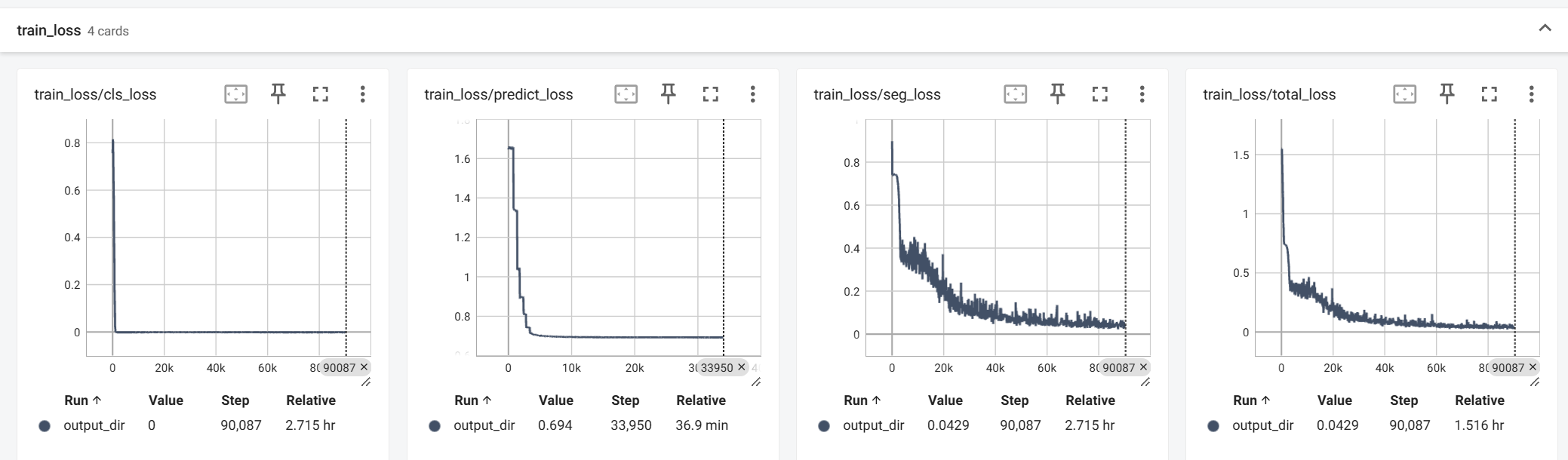
The calculation of the evaluation metrics comes from the results of pred_mask and pred_label and is obtained by calculating with mask:
![]()
The visualization of the predicted results, obtained from the visual_image field, and the default input images such as image, mask are also automatically visualized and output, which can be used to directly observe where the model's current predictions are not good, facilitating further model improvement.
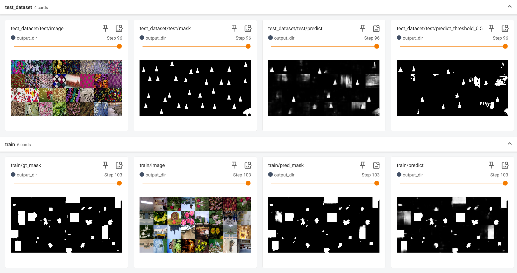
Note
The tutorial should have image samples here. If you do not see the images, please check your network connection or enable VPN.
All the weights obtained after training (Checkpoint) are saved in the path corresponding to base_dir at the beginning of the training train_mymodel.sh script. The log files of Tensorboard are also saved here for subsequent use and log review.
In addition to Tensorboard logs, we also provide a plain text log log.txt for archiving, which contains simple content, including all scalar information after each Epoch. An example is as follows:
......
{"train_lr": 5.068414063259753e-05, "train_total_loss": 0.040027402791482446, "train_seg_loss": 0.04001608065957309, "train_cls_loss": 1.1322131909352606e-05, "test_pixel-level F1": 0.6269838496863315, "epoch": 100}
{"train_lr": 4.9894792537480576e-05, "train_total_loss": 0.03938291078949974, "train_seg_loss": 0.039372251576574625, "train_cls_loss": 1.0659212925112626e-05, "epoch": 101}
{"train_lr": 4.910553386394297e-05, "train_total_loss": 0.039195733024078264, "train_seg_loss": 0.039184275720948555, "train_cls_loss": 1.1457303129702722e-05, "epoch": 102}
{"train_lr": 4.8316563303634596e-05, "train_total_loss": 0.0385435631179897, "train_seg_loss": 0.03853294577689024, "train_cls_loss": 1.061734109946144e-05, "epoch": 103}
{"train_lr": 4.752807947567499e-05, "train_total_loss": 0.035692626619510615, "train_seg_loss": 0.03568181328162471, "train_cls_loss": 1.0813337885906548e-05, "test_pixel-level F1": 0.6672104743469334, "epoch": 104}
The model is tested every 4 Epochs, so only the corresponding epoch will save test_pixel-level F1.
Thus, we have explained all the output content during the training process.
Conducting Tests
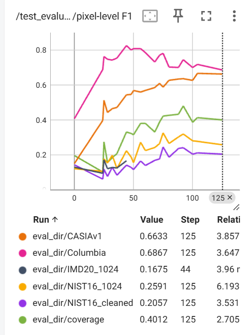
We saw in the previous metric tests that the model still had an upward trend at the 104th Epoch, but to save time, we stopped training here and proceeded to subsequent tests.
The gap between tamper detection datasets is quite large, and generalization performance is the most important indicator to measure model performance, so we hope to measure all indicators at once. Unlike previous tutorials, we need to use the test_datasets.json file that can cover multiple test datasets at once to assist in testing. The format is as follows, and we also provide a sample of this file in the files after benco init.
{
    "Columbia": "/mnt/data0/public_datasets/IML/Columbia.json",
    "NIST16_1024": "/mnt/data0/public_datasets/IML/NIST16_1024",
    "NIST16_cleaned": "/mnt/data0/public_datasets/IML/NIST16_1024_cleaning",
    "coverage": "/mnt/data0/public_datasets/IML/coverage.json",
    "CASIAv1": "/mnt/data0/public_datasets/IML/CASIA1.0",
    "IMD20_1024": "/mnt/data0/public_datasets/IML/IMD_20_1024"
}
You need to preprocess each dataset in advance, and the dataset index is in the Tamper Detection Dataset Index section, and the format requirements are in the Dataset Preparation Section. The above paths must be organized in the format of ManiDataset or JsonDataset.
Then we modify the test_mymodel.sh file to pass in the correct parameters, mainly including the following fields:
- Change
--mymodeltoMyConvNeXt - Remove unnecessary
--MyModel_Customized_paramand--pre_trained_weightsespeciallypretrained_pathis usually initialized before model training. It is irrelevant during the testing phase. - Set
--checkpoint_pathto the folder where allcheckpoint-xx.pthare output during training. It will automatically read all files ending with.pthunder this folder and determine which epoch the checkpoint comes from based on the number in the filename to correctly plot the test metrics line chart. - Set
--test_data_jsonto the path of the JSON containing multiple test set information mentioned earlier. - Other parameters can be set according to the memory and other conditions as appropriate,
Note
If you chose --if_padding during training, this means that the dataloader will organize all images in the 0-padding manner of IML-ViT, not the --if_resizing of most models. Then make sure that this parameter is consistent between training and testing, otherwise, there will definitely be performance loss due to the inconsistency between the training set and the test set.
You can double-check whether padding or resizing is correctly selected through the pictures visualized by Tensorboard!
A modified test_mymodel.sh is as follows:
base_dir="./eval_dir"
mkdir -p ${base_dir}

CUDA_VISIBLE_DEVICES=0,1 \
torchrun  \
    --standalone    \
    --nnodes=1     \
    --nproc_per_node=2 \
./test.py \
    --model MyConvNeXt \
    --world_size 1 \
    --test_data_json "./test_datasets.json" \
    --checkpoint_path "./output_dir/" \
    --test_batch_size 32 \
    --image_size 512 \
    --if_resizing \
    --output_dir ${base_dir}/ \
    --log_dir ${base_dir}/ \
2> ${base_dir}/error.log 1>${base_dir}/logs.log
Then, remember to change from mymodel import MyModel at the beginning of test.py to from mymodel import MyConvNeXt.
At this point, running the following command can start batch testing metrics on various test sets:
sh test_mymodel.sh
At this time, you can also view the test progress and results through Tensorboard. You can filter eval_dir in the filter box on the left to only view the output results of this test.
tensorboard --logdir ./
The line charts of metrics obtained from multiple datasets after testing are as follows. Choose the Checkpoint with the best comprehensive performance and record the corresponding data in the paper.
Robustness Testing
Robustness testing introduces two dimensions of "attack type" and "attack strength" for grid search (gird search), so it is generally only the best-performing checkpoint during the test phase that undergoes robustness testing.
Accordingly, in the test_robust_mymodel.sh file, unlike test_mymodel.sh, the --checkpoint_path field here points to a specific checkpoint, not a folder.
The other fields are the same, remove unnecessary parameters, fill in the required parameters, and remember to change from mymodel import MyModel at the beginning of test_robust.py to from mymodel import MyConvNeXt.
The test_robust_mymodel.sh I finally used is as follows:
base_dir="./eval_robust_dir"
mkdir -p ${base_dir}

CUDA_VISIBLE_DEVICES=0,1 \
torchrun  \
    --standalone    \
    --nnodes=1     \
    --nproc_per_node=2 \
./test_robust.py \
    --model MyConvNeXt \
    --world_size 1 \
    --test_data_path "/mnt/data0/public_datasets/IML/CASIA1.0" \
    --checkpoint_path "/mnt/data0/xiaochen/workspace/IMDLBenCo_pure/guide/benco/output_dir/checkpoint-92.pth" \
    --test_batch_size 32 \
    --image_size 512 \
    --if_resizing \
    --output_dir ${base_dir}/ \
    --log_dir ${base_dir}/ \
2> ${base_dir}/error.log 1>${base_dir}/logs.log
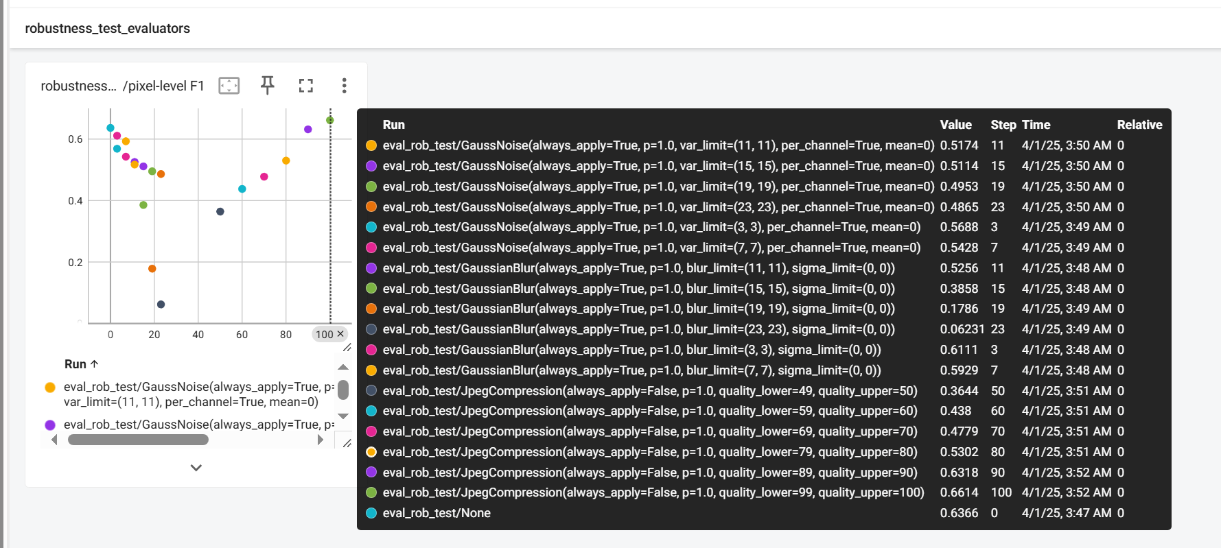
The specific adjustment of attack strategies and intensities in robustness testing requires modification of test_robust.py. Please locate this modifiable code by searching for TODO:
    """=================================================
    Modify here to Set the robustness test parameters TODO
    ==================================================="""
    robustness_list = [
            GaussianBlurWrapper([0, 3, 7, 11, 15, 19, 23]),
            GaussianNoiseWrapper([3, 7, 11, 15, 19, 23]),
            JpegCompressionWrapper([50, 60, 70, 80, 90, 100])
    ]
The lists behind these wrapper represent the specific strengths of the attacks, and they internally encapsulate the Transform provided by Albumentation to implement the attack. The implementation of the wrapper itself, please refer to this link.
In particular, you can refer to the implementation of the wrapper in the current path to encapsulate a new custom wrapper, and then import your own wrapper here like from mymodel import MyConvNeXt. This way, you can achieve a custom flexible robustness test without modifying the source code.
For test results, similarly, you can view them through Tensorboard:
tensorboard --logdir ./
At this time, there may be many different records. Please make good use of the filter function in the upper left corner of Tensorboard to filter the attack types and corresponding results you need to record.
Conclusion
In this way, we have completed the process of designing a model from scratch, training the model, completing testing and robustness testing. If you have any questions or incomplete places, please feel free to raise issues in our repository or contact the author team by email. The suggestions from the first-hand users will be of great help to us and to future scholars!